
Quick Links
- Why another query language?
- Concrete examples
- Can the query DSL do the same?
- What else do we have in store?
- Limitations
- Conclusion
Why another query language?
In the beginning, Elastic created the almighty query DSL: a powerful, flexible, and very expressive language to query your Elasticsearch data using JSON-formatted queries. With the query DSL, the possibilities are limitless as you can mix and match your queries in pretty much any way you like. However, this high flexibility also came with increased complexity, meaning it was not always easy for any newcomer to come up with an optimal query in a reasonable amount of time. In very early versions, it was important to build your queries the “right way,” i.e., prefer filters, arrange them in a specific order, etc.
Gradually, Elasticsearch became smarter at parsing and executing your queries, and the constraints on how you had to build your queries were relaxed. Eventually, new query languages came to life, such as EQL and SQL in Elasticsearch and KQL and Timelion in Kibana. Not only were each of those languages created to serve a very specific purpose but they also all transpiled their high-level queries into low-level DSL queries underneath.
The new ES|QL query language takes a completely different approach. It has been built from the ground up to query any kind of data indexed in Elasticsearch, but more importantly, the query engine doesn’t convert the queries to the query DSL at all. This means that an ES|QL query doesn’t use the same query and aggregation infrastructure as the DSL queries and is run by a completely dedicated querying engine that was built with multi-threading and performance in mind.
After more than one year of development, the new ES|QL feature was released in 8.11 and enables new use cases that are more difficult to achieve with existing features, such as log exploration, threat hunting, etc. If you have heard about or used Splunk’s SPL (Search Processing Language) or OpenSearch’s PPL (Piped Processing Language), ES|QL can be considered as Elastic’s response to them.
Let’s look at some concrete examples
Instead of digging straight into the detail of the syntax, it probably helps to provide a quick example that illustrates what an ES|QL query looks like. Let’s take a sample query used in a recent blog article which works over the MySQL sample employees data set:
POST _query?format=txt
{
  "query": """
  FROM employees
| EVAL hired_year = TO_INTEGER(DATE_FORMAT("YYYY", hire_date))
| WHERE hired_year > 1985
| STATS avg_salary = AVG(salary) BY languages
| EVAL avg_salary = TO_INTEGER(ROUND(avg_salary))
| EVAL lang_code = TO_STRING(language)
| ENRICH languages_policy ON lang_code WITH lang = language_name
| WHERE lang IS NOT NULL
| KEEP avg_salary, lang
| SORT avg_salary ASC
| LIMIT 3
  """
}
Note: Much like the aforementioned languages (i.e., SPL and PPL), ES|QL is also a piped language, hence the pipe in its name. Pipes are nothing new as they were initially invented in the 1970s to enable inter-process communication in the Unix operating system.
Back to our sample query above, we can see different blocks separated by pipes wrapped as a string passed into the `query` section (line 3) and sent to the `_query` API endpoint (line 1).
At the beginning of the query, we have a source command (e.g., `FROM` on line 4) which provides the data to be processed by the subsequent processing commands (lines 5–14). Each processing block is executed sequentially from top to bottom, and the result of one block is passed as an input to the next block. Moreover, the query is pretty easy to read as most of the commands are common English nouns, verbs, or abbreviations thereof, pretty much like with SQL. Reading through it, we can easily grasp what the query does, i.e., computing the lowest three average salaries by employee language.
In the upcoming sections, we are going to illustrate step-by-step how the above query is executed and what the data looks like at each step in the process.
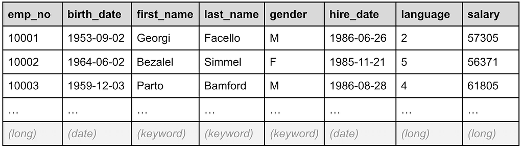
Line 4. FROM employees
The FROM source command retrieves the first 500 documents from the `employees` index in no specific order, as shown in Table 1, below. Note that the last row is not part of the output, but we have added it so that we can show what data type each column contains.
Table 1: The FROM source command retrieves the data to be processed
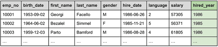
Line 5. EVAL hired_year = TO_INTEGER(DATE_FORMAT(“YYYY”, hire_date))
Table 2, below, shows how the next EVAL processing command creates for each record a new field called `hired_year`, which is the year component of the `hire_date` field value.
Table 2: The EVAL command creates a new hired_year field
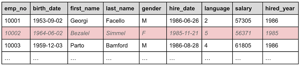
Line 6. WHERE hired_year > 1985
The next WHERE processing command filters out all records whose newly created `hired_year` field is smaller than or equal to 1985. The record 10002 is now removed from the data set, as we can see in Table 3, below:
Table 3: The WHERE command filters out records with hired_year > 1985
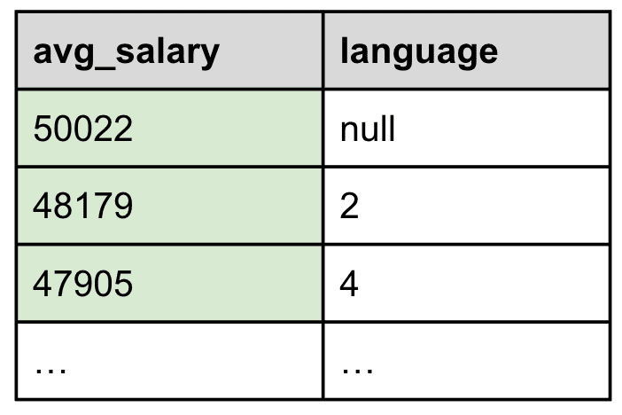
Line 7. STATS avg_salary = AVG(salary) BY languages
The next line is where it gets interesting as we start aggregating data. From all the remaining documents not filtered out by the previous WHERE command, the STATS … BY… processing command will group them by their `languages` column and create a new field called `avg_salary` containing the average of all salaries for each language in long format. Table 4, below, shows the new face of the result set as we are aggregating the whole data set:
Table 4: The STATS command groups by language and computes the average salary

As we will see shortly, since there are five different languages the new table can only have six different rows, i.e., one for each language and one for all employee records without any language specified.
Line 8. EVAL avg_salary = TO_INTEGER(ROUND(avg_salary))
We now want to clean up the data, and the first task is to round the average salary figures. The next EVAL processing command redefines the `avg_salary` field by rounding its value up or down to the closest number and casting it to an integer value, as we can see in Table 5, below:
Table 5: The average salary field is rounded to the nearest integer number
Line 9. EVAL lang_code = TO_STRING(language)
This next step is a technical one, though it helps highlight a nice and powerful capability of ES|QL, as we’ll see shortly. What we want to carry out now is to map each language identifier to the real language name, so that we show “English” instead of “1”, “French” instead of “2”, etc. To achieve this, we’re going to leverage a great feature supported by Elasticsearch that can enrich our data with data from another index.
To be able to enrich our data with the spelled-out language name, we need to join our current data with another index called `languages`, which contains a mapping of the language identifier to the corresponding language name, as shown in Table 6, below:
Table 6: The languages table contains a list of languages
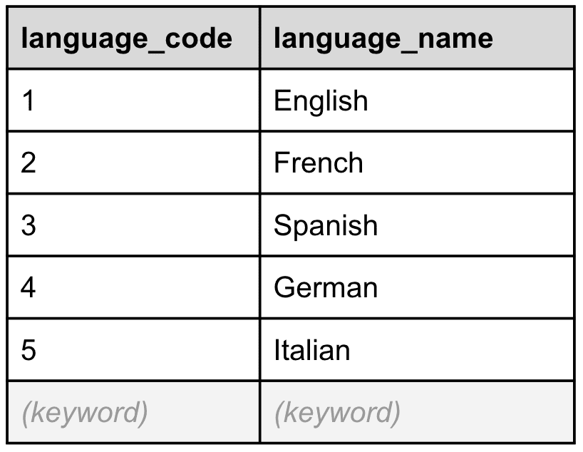
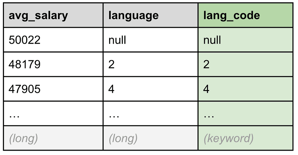
To sum up, we want to join the `language` field from the data set we got from the execution of line 8 with the `language_code` field from the `languages` table above. However, this will only work if the joined fields have the same data type, and as we can see, `language` is a long, while `language_code` is a keyword.
No big deal, ES|QL has you covered. In Table 7, below, we can see how the next EVAL processing command creates a new keyword field called `lang_code` containing a stringified version of the `language` field. We will now be able to join this new `lang_code` field with the `language_code` field we just saw in Table 6.
Table 7: A new `lang_code` keyword field has been created to perform the join later
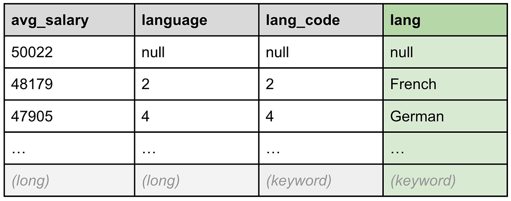
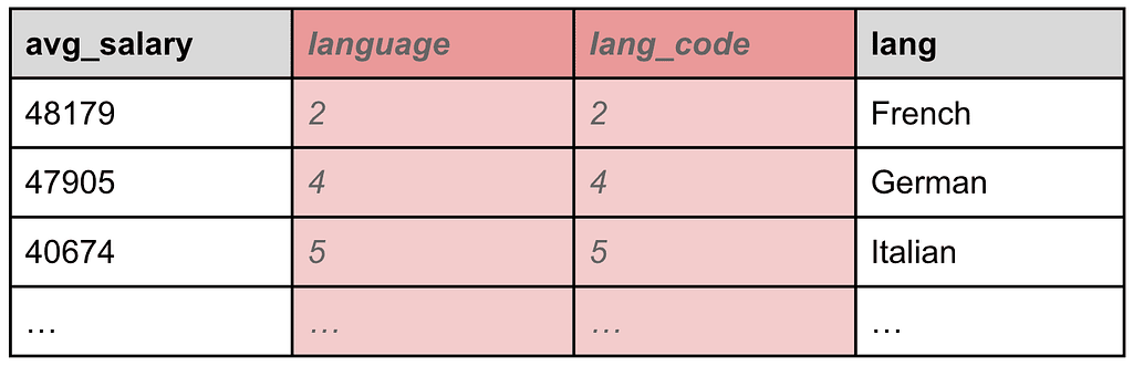
Line 10. ENRICH languages_policy ON lang_code WITH lang = language_name
For the enrichment step, we will now be able to rely on a pre-existing “exact match” enrich policy called `languages_policy` that has been built on the `languages` table we showed in the previous section. Without going too much into the details, the `languages_policy` enrich policy creates a hidden enrichment index keyed on the `language_code` field that can be used as a JOIN table. This enrich policy must be created prior to running the query, but don’t worry, Kibana will allow you to create one dynamically as it detects that none exists.
The ENRICH … ON … WITH … processing command leverages this enrichment policy to find a match for each `lang_code` value. When it finds them, it creates a new field called `lang` containing the value of the `language_name` field of the matched language record, as shown in Table 8, below:
Table 8: A new lang field with the spelled-out language name has been added
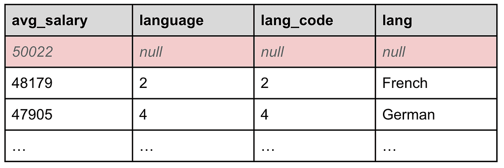
Line 11. WHERE lang IS NOT NULL
We are almost there, but some cleanup is now in order. We now want to get rid of the average salary for which there is no language information. For that, we use another WHERE command to filter out all records whose `lang` field is null, i.e., the first one, as shown in Table 9, below:
Table 9: The row with no language information is filtered out
At this point, it is interesting to note that all the filtering doesn’t necessarily need to happen at the same time in the same or subsequent WHERE blocks; it can be performed at various points in time during the execution to include or exclude records as the data gets transformed along the way.
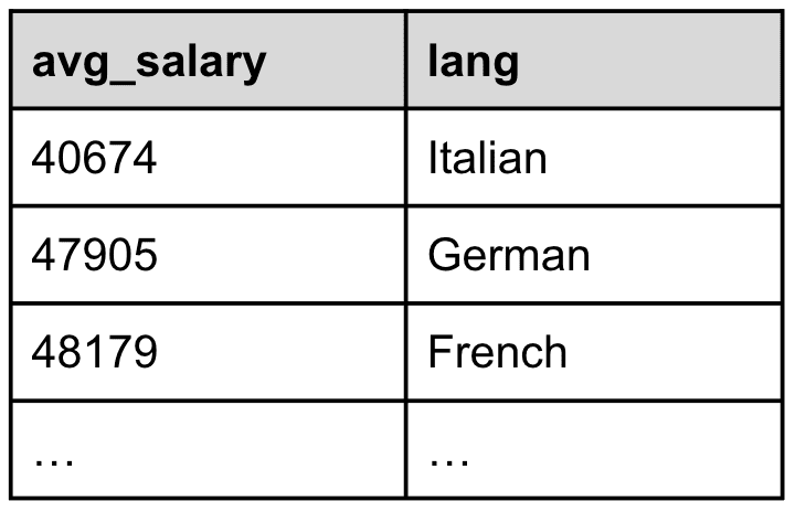
Line 12. KEEP avg_salary, lang
Now that we are done transforming, filtering, and joining our data, we can prepare the final result set by removing the temporary fields we have created along the way. The KEEP command allows us to specify exactly which fields we want to let go through. All the other ones will be pruned, as shown in Table 10, below:
Table 10: Unneeded fields are pruned
Another command named DROP (not used here) performs the opposite action, i.e., it prunes the specified fields and keeps all the other ones. You can use either command depending on how many fields you want to keep or prune.
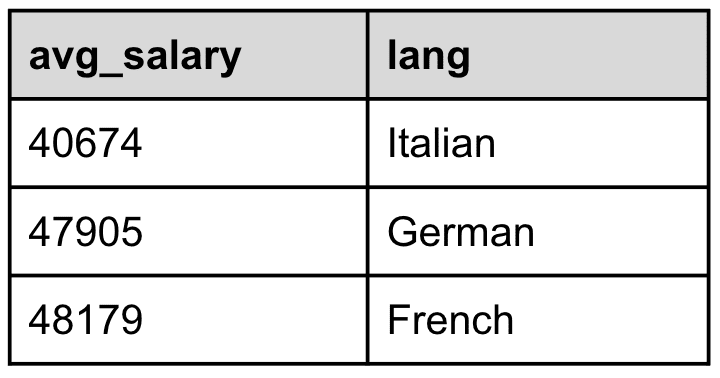
Line 13. SORT avg_salary ASC
We also want to sort our final result set by ascending average salary figures, and that can be easily done with the SORT … ASC processing command, as shown in Table 11, below:
Table 11: The average salary figures are sorted from the lowest to the highest
Regarding the SORT command, the two valid modes are DESC and ASC, which is the default mode if no mode is specified.
Line 14. LIMIT 3
Finally, we only want to show the languages for the lowest three average salary figures, and the LIMIT processing command helps us do that, as shown in Table 12, below:
Table 12: Only the three languages with the lowest average salary are selected in the result set
Wow, that was quite a ride, wasn’t it? We went all the way from sourcing data, filtering by year, looking up and aggregating by language names, computing the average salary by language group, creating new fields, pruning unneeded ones, sorting by average salaries, and finally limiting the result set. Pretty amazing what we managed to do with a single query made of eleven lines of code. Now, onto the next question…
Can the query DSL do the same?
Needless to say, it is not possible to achieve the same with a single DSL query. Enrichment, for instance, can only happen at indexing time by leveraging an ingest pipeline composed of an enrich processor, which means that you need to know beforehand when indexing your data what you might want to join with it later in your query. Regardless, you first need to store the joined data in your index in order to be able to query it later, there’s no way around that. In this case, we would need to store the language name inside our `employees` documents at indexing time so that we can then aggregate and filter on it.
Creating fields on the fly and filtering on them can be done with runtime fields, but their usage at query time is pretty limited, especially when trying to transform their values using functions at aggregations time. Pruning fields, especially ones created in aggregations, is not possible with the conventional query DSL.
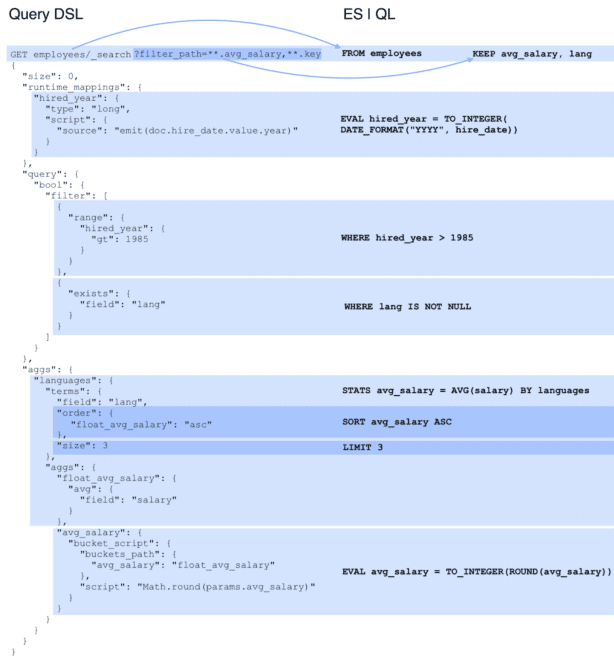
We’ve attempted to create a DSL query that returns the same data as the above query, and we came up with the one in Figure 1, below. As you can see, lines 9 and 10 (ENRICH) are missing because the query DSL doesn’t provide similar functionality for query-time enrichment. It is also worth noting that we had to update the index in order to enrich it with the language names so that we could filter and aggregate on them. Also, it’s much longer and more verbose, and the query flow is not as intuitive as when reading the original ES|QL query.
Figure 1: A remotely equivalent DSL query
The response we get from the above DSL query contains exactly the same result set, however, there’s no way to rename the language keys as can be seen in Figure 2, below:
Figure 2: The results from the DSL query
In conclusion, while with ES|QL everything happens at query time, trying to achieve the same with the query DSL involves some pre-enrichment tasks at indexing time and additional client code to massage the result set since it’s not possible to transform the JSON response from Elasticsearch.
What else do we have in store?
Response formatting
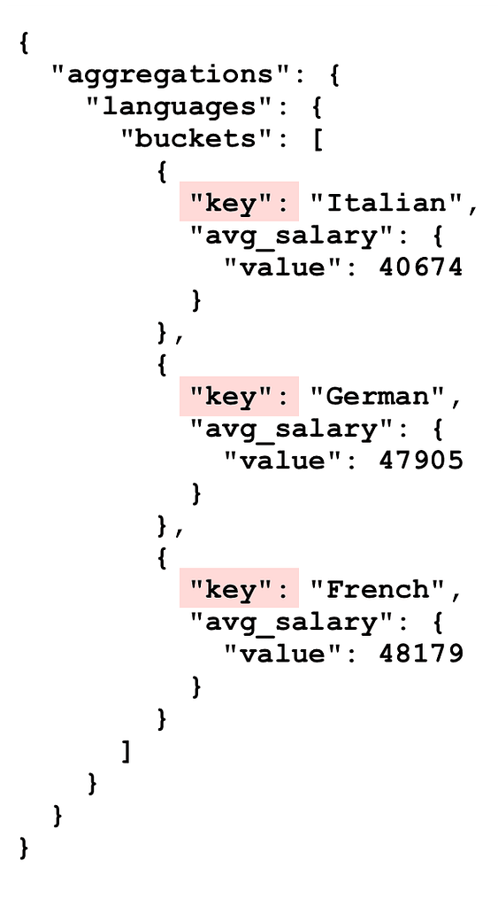
Using the `format` query string parameter, a DSL query response can be returned as either JSON (default), YAML, CBOR, or SMILE. A great addition brought by ES|QL is the ability to format the response in more readable formats, such as the TXT format that we have used in the example above which returns data in a formatted table. Other useful formats include CSV and TSV, which return the results in comma-delimited and tab-delimited formats, respectively, ready to be consumed by other applications or imported into spreadsheets. An example of a CSV output is shown in the code below:
avg_salary,lang
40674,Italian
47905,German
48179,French
ES|QL also supports the other binary formats, such as CBOR and SMILE. Moreover, it is obviously also possible to return the data as JSON and YAML but in a columnar format, which looks slightly different from what the DSL query returns, as can be seen in the code below:
{
  "columns": [
    { "name": "avg_salary", "type": "integer" },
    { "name": "lang", "type": "keyword" }
  ],
  "values": [
    [ 40674, "Italian" ],
    [ 47905, "German" ],
    [ 48179, "French" ]
  ]
}
The JSON format also supports a second mode when turning on the `columnar` flag in the query payload. In that mode, each row will contain all the values of a certain column in the results, as shown in the code below:
POST _query?format=txt
{
  "columnar": true,
  "query": """
    ...
  """
}

=>
{
  "columns": [
    { "name": "avg_salary", "type": "integer" },
    { "name": "lang", "type": "keyword" }
  ],
  "values": [
    [ 40674, 47905, 48179 ],
    [ "Italian", "German", "French" ]
  ]
}
Filtering
While ES|QL provides filtering capabilities through the use of the WHERE command, it is also possible to add additional filters using the conventional query DSL using the `filter` section, as shown in the following code:
POST _query?format=txt
{
  "query": """
    ...
  """,
  "filter": {
    "range": {
      "salary": {
        "gt": 10000
      }
    }
  }
}
Query parameters
Sometimes, it might come in handy to not hardcode values into your query and be able to pass them as parameters. In the following code, we can see how the `hired_year` threshold and the limit have been parameterized and the actual values are being passed in the `params` array. It is worth noting that such parameterized queries also protect you from any hacking or code injection, so it’s a good practice to proceed that way.
POST _query?format=txt
{
  "query": """
  FROM employees
| EVAL hired_year = TO_INTEGER(DATE_FORMAT("YYYY", hire_date))
| WHERE hired_year > ?
... commands omitted for brevity
| LIMIT ?
  """,
  "params": [1985, 3]
}
Limitations
Every new feature comes with some limitations, and ES|QL is no exception to that rule. The first limitation concerns the size of the result set. Whatever number is specified in the LIMIT command, the result set will never contain more than 10,000 documents.
The second limitation relates to the supported data types. Not all data types are supported, but the most common ones are, such as text, keyword, date, boolean, double, etc. You can consult the official documentation to find out the complete list of data types supported by ES|QL.
Conclusion
We have only scratched the surface of what the new ES|QL query language allows us to do. There are a few more commands that we haven’t shown here, such as the ability to dynamically DISSECT or GROK arbitrary strings according to a pattern. Also, there are many more functions for doing math, manipulating strings, formatting and parsing dates, converting types, operating on multi-valued fields, and so on.
We encourage you to check out the official ES|QL documentation and start experimenting on your own data, you’ll be amazed at the tons of new possibilities you can unlock. If you need some inspiration, don’t hesitate to check out some other example queries provided in the Elastic AI Assistant knowledge base and also check out Elastic’s official announcement that provides even more insights on how to leverage ES|QL inside Kibana.