
Quick links
- Overview
- The need for hybrid search
- Timeline
- The anatomy of hybrid search in Elasticsearch
- Let’s conclude
Overview
This article is the last one in a series of five that dives into the intricacies of vector search (aka semantic search) and how it is implemented in OpenSearch and Elasticsearch.
The first part: A Quick Introduction to Vector Search, was focused on providing a general introduction to the basics of embeddings (aka vectors) and how vector search works under the hood. The content of that article was more theoretical and not oriented specifically on OpenSearch, which means that it was also valid for Elasticsearch as they are both based on the same underlying vector search engine: Apache Lucene.
Armed with all the vector search knowledge learned in the first article, the second article: How to Set Up Vector Search in OpenSearch, guided you through the meanders of how to set up vector search in OpenSearch using either the k-NN plugin or the new Neural Search plugin that was recently made generally available in 2.9.
In the third part: OpenSearch Hybrid Search, we leveraged what we had learned in the first two parts and built upon that knowledge by delving into how to craft powerful hybrid search queries in OpenSearch.
The fourth part: How to Set Up Vector Search in Elasticsearch, was similar to the second one but focused on how to set up vector search and execute k-NN searches in Elasticsearch specifically.
This last part is similar to the third one but focuses on running hybrid search queries in Elasticsearch.
The need for hybrid search
Before diving into the realm of hybrid search, let’s do a quick refresh of what we learned in the first article of this series regarding how lexical and semantic search differ and how they can complement each other.
To sum it up very briefly, lexical search is great when you have control over your structured data and your users are more or less clear on what they are searching for. Semantic search, however, provides great support when you need to make unstructured data searchable and your users don’t really know exactly what they are searching for. It would be fantastic if there was a way to combine both together in order to squeeze as much substance out of each one as possible. Enter hybrid search!
In a way, we can see hybrid search as some sort of “sum” of lexical search and semantic search. However, when done right, hybrid search can be much better than just the sum of those parts, yielding far better results than either lexical or semantic search would do on their own.
Running a hybrid search query usually boils down to sending a mix of at least one lexical search query and one semantic search query and then merging the results of both. The lexical search results are scored by a similarity algorithm, such as BM25 or TF-IDF, whose score scale is usually unbounded as the max score depends on the number and frequency of terms stored in the inverted index. In contrast, semantic search results can be scored within a closed interval, depending on the similarity function that is being used (e.g., [0; 2] for cosine similarity).
In order to merge the lexical and semantic search results of a hybrid search query, both result sets need to be fused in a way that maintains the relative relevance of the retrieved documents, which is a complex problem to solve. Luckily, there are several existing methods that can be utilized; two very common ones are Convex Combination (CC) and Reciprocal Rank Fusion (RRF).
Basically, Convex Combination, also called Linear Combination, seeks to combine the normalized score of lexical search results and semantic search results with respective weights and (where 0 ,), such that:

CC can be seen as a weighted average of the lexical and semantic scores, but in contrast to OpenSearch, the weights are not expressed as percentages, i.e., they do not need to add up to 100%. Weights between 0 and 1 are used to deboost the related query, while weights greater than 1 are used to boost it.
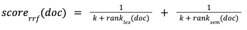
RRF, however, doesn’t require any score calibration or normalization and simply scores the documents according to their rank in the result set, using the following formula, where k is an arbitrary constant meant to adjust the importance of lowly ranked documents:
Both CC and RRF have their pros and cons as highlighted in Table 1, below:
Table 1: Pros and cons of CC and RRF
| Convex Combination | Reciprocal Rank Fusion | |
|---|---|---|
| Pros | - Good calibration of weights makes CC more effective than RRF | - Doesn’t require any calibration - Fully unsupervised - No need to know min/max scores |
| Cons | - Requires a good calibration of the weights - Optimal weights are specific to each data set | - Not trivial to tune the value of k - Ranking quality can be affected by increasing result set size |
It is worth noting that not everyone agrees on these pros and cons depending on the assumptions being made and the data sets on which they have been tested. A good summary would be that RRF yields slightly less accurate scores than CC but has the big advantage of being “plug & play” and can be used without having to fine-tune the weights with a labeled set of queries.
In contrast to OpenSearch, which went hybrid the CC way as of version 2.10, Elastic decided to support both the CC and RRF approaches. We’ll see how this is carried out later in this article. If you are interested in learning more about the rationale behind that choice, you can read this great article from the Elastic blog and also check out this excellent talk on RRF presented at Haystack 2023 by Elastician Philipp Krenn.
Timeline
As mentioned in the previous article, Elasticsearch came late into the vector search game and only started supporting approximate nearest neighbors (ANN) search in February 2022 with the 8.0 release. In contrast, OpenDistro for Elasticsearch already released that feature in September 2019 via their k-NN plugin for Elasticsearch 7.2, shortly after Apache Lucene started to support dense vectors.
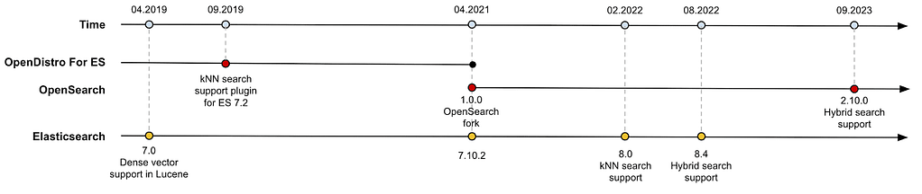
Even though Elasticsearch was more than two years behind OpenDistro/OpenSearch in terms of ANN support, they caught up extremely rapidly, and in just a few months, they managed to provide hybrid search support with the 8.4 release in August 2022. OpenSearch, however, released support for hybrid search only in September 2023 with the release of 2.10. Figure 1, below, shows the OpenSearch and Elasticsearch timelines for bringing hybrid search to market:
Figure 1: Hybrid search timeline for OpenSearch and Elasticsearch
The anatomy of hybrid search in Elasticsearch
As we’ve briefly hinted at in our previous article, vector search support in Elasticsearch has been made possible by leveraging dense vector models (hence the `dense_vector` field type), which produce vectors that usually contain essentially non-zero values and represent the meaning of unstructured data in a multi-dimensional space.
However, dense models are not the only way of performing semantic search. Elasticsearch also provides an alternative way that uses sparse vector models. Elastic created a sparse NLP vector model called Elastic Learned Sparse EncodeR, or ELSER for short, which is an out-of-domain (i.e., not trained on a specific domain) sparse vector model that does not require any fine-tuning. It was pre-trained on a vocabulary of approximately 30,000 terms, and as it’s a sparse model most of the vector values (i.e., more than 99.9%) are zeros.
The way it works is pretty simple. At indexing time, the sparse vectors containing term/weight pairs are generated using the `inference` ingest processor and stored in fields of type `rank_features`, which is the sparse counterpart to the `dense_vector` field type. At query time, a specific DSL query called `text_expansion` replaces the original query terms with terms available in the ELSER model vocabulary that are known to be the most similar to them given their weights.
Sparse or dense?
Before heading over to hybrid search queries, we would like to briefly highlight the differences between sparse and dense models. Figure 2, below, shows how the piece of text “the quick brown fox” is encoded by each model.
In the sparse case, the four original terms are expanded into 30 weighted terms that are closely or distantly related to them. The higher the weight of the expanded term, the more related it is to the original term. Since the ELSER vocabulary contains more than 30,000 terms, it means that the vector representing “the quick brown fox” has as many dimensions and contains only ~0.1% of the non-zero values (i.e., ~30 / 30,000), hence why we call these models sparse.
Figure 2: Comparing sparse and dense model encoding
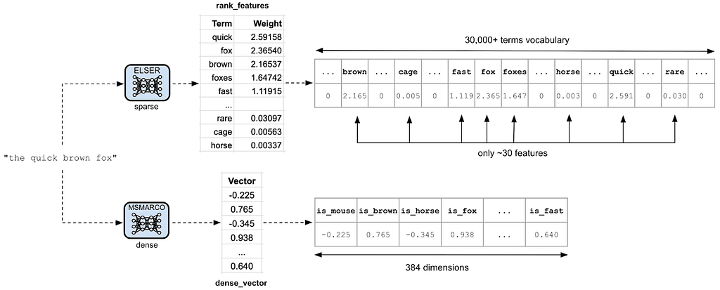
In the dense case, “the quick brown fox” is encoded into a much smaller embeddings vector that captures the semantic meaning of the text. Each of the 384 vector elements contains a non-zero value that represents the similarity between the piece of text and each of the dimensions. Note that the names we have given to dimensions (i.e., `is_mouse`, `is_brown`, etc.) are purely fictional, and their purpose is just to give a concrete description of the values.
Another important difference is that sparse vectors are queried via the inverted index (yes, like lexical search), whereas as we have seen in previous articles, dense vectors are indexed in specific graph-based or cluster-based data structures that can be searched using approximate nearest neighbors algorithms.
We won’t go any further into the details of how ELSER came to be, but if you’re interested in understanding how that model was born, we recommend you check out this article from the Elastic Search Labs, which explains in detail the thought process that led Elastic to develop it. If you are thinking about evaluating ELSER, it might be worth checking Elastic’s relevance workbench, which demonstrates how ELSER compares to a normal BM25 lexical search. We are also not going to dive into the process of downloading and deploying the ELSER model in this article, but you can take a moment and turn to the official documentation that explains very well how to do it.
Hybrid search support
Whether you are going to use dense or sparse retrieval, Elastic provides hybrid search support for both model types. The first type is a mix of a lexical search query specified in the `query` search option and a vector search query (or an array thereof) specified in the `knn` search option. The second one introduces a new search option called `sub_searches` which also contains an array of search queries that can be of lexical (e.g., `match`) or semantic (e.g., `text_expansion`) nature.
If all this feels somewhat abstract to you, don’t worry, as we will shortly dive into the details to show how hybrid searches work in practice and what benefits they provide.
Hybrid search with dense models
This is the first hybrid search type we just mentioned. It basically boils down to running a lexical search query mixed with an approximate k-NN search in order to improve relevance. Such a hybrid search query is shown below:
POST my-index/_search
{
  "size": 10,
  "_source": false,
  "fields": [ "price" ],
  "query": {
    "bool": {
      "must": [
        {
          "match": {
            "text-field": {
              "query": "fox",
              "boost": 0.2
            }
          }
        }
      ]
    }
  },
  "knn": {
    "field": "title_vector",
    "query_vector": [0.1, 3.2, 2.1],
    "k": 5,
    "num_candidates": 100,
    "boost": 0.8
  }
}
As we can see above, a hybrid search query is simply a combination of a lexical search query (e.g., a `match` query) located in the `query` section and a vector search query specified in the `knn` section. What this query does is first retrieve the top five vector matches at the global level, then combine them with the lexical matches, and finally return the ten best matching hits. The way vector and lexical matches are combined is through a disjunction (i.e., a logical OR condition) where the score of each document is computed using Convex Combination, i.e. the weighted sum of its vector and lexical scores, as we saw earlier.
Elasticsearch also provides support for running the exact same hybrid query using RRF ranking instead, which you can do by simply specifying an additional `rank` section in the query payload, as shown below:
POST my-index/_search
{
  "size": 10,
  "_source": false,
  "fields": [ "price" ],
  "query": {
    "...":
  },
  "knn": {
    "...":
  },
  "rank": {
    "rrf": {
      "rank_constant": 60,
      "window_size": 100
    }
  }
}
This query runs pretty much the same way as earlier, except that `window_size` documents (e.g., 100 in this case) are retrieved from the vector and lexical queries and then ranked by RRF instead of being scored using CC. Finally, the top documents ranked from 1 to `size` (e.g., 10) are then returned in the result set.
The last thing to note about this hybrid query type is that RRF ranking requires a commercial license (Platinum or Enterprise), but if you don’t have one, you can still leverage hybrid searches with CC scoring or by using a trial license that allows you to enjoy the full feature set for one month.
Hybrid search with sparse models
The second hybrid search type for querying sparse models works with another search option called `sub_searches`. Newly introduced in version 8.9, it basically replaces the `query` section and allows users to specify an array of lexical and semantic queries (e.g., `text_expansion`) that will be independently executed, and whose results are going to be ranked together. Below, we can see what such a hybrid query looks like:
POST my-index/_search
{
  "_source": false,
  "fields": [ "text-field" ],
  "sub_searches": [
    {
      "query": {
        "match": {
          "text-field": "fox"
        }
      }
    },
    {
      "query": {
        "text_expansion": {
          "ml.tokens": {
            "model_id": ".elser_model_1",
            "model_text": "a quick brown fox jumps over a lazy dog"
          }
        }
      }
    }
  ],
  "rank": {
    "rrf": {}
  }
}
In the above query, we can see that the `sub_searches` array contains one lexical `match` query as well as one semantic `text_expansion` query that works on the ELSER sparse model that we introduced earlier.
It is also worth noting that when specifying `sub_searches` to run hybrid queries, it is mandatory to include the `rank` section to leverage RRF ranking. Hence, this feature is only available with a commercial license (or a trial license valid for one month).
Hybrid search with dense and sparse models
So far, we have seen two different ways of running a hybrid search, depending on whether a dense or sparse vector space was being searched. At this point, you might wonder whether we can mix both dense and sparse data inside the same index, and you’ll be pleased to learn that it is indeed possible. One concrete application could be that you need to search both a dense vector space with images and a sparse vector space with textual descriptions of those images. Such a query would look like this:
POST my-index/_search
{
  "_source": false,
  "fields": [ "text-field" ],
  "query": {
    "text_expansion": {
      "ml.tokens": {
        "model_id": ".elser_model_1",
        "model_text": "a quick brown fox jumps over a lazy dog",
        "boost": 0.5
      }
    }
  },
  "knn": {
    "field": "image-vector",
    "query_vector": [0.1, 3.2, ..., 2.1],
    "k": 5,
    "num_candidates": 100,
    "boost": 0.5
  }
}
In the above payload, we can see two equally weighted queries, namely a `text_expansion` query searching for image descriptions within the ELSER sparse vector space, and in the `knn` section a vector search query searching for image embeddings (e.g., “brown fox” represented as an embedding vector) in a dense vector space. In addition, you can also leverage RRF by providing the `rank` section at the end of the query.
You can even add a lexical search query to the mix using the `sub_searches` section we introduced earlier, and it would look like this:
POST my-index/_search
{
  "_source": false,
  "fields": [ "text-field" ],
  "sub_searches": [
    {
      "query": {
        "match": {
          "text-field": "brown fox"
        }
      }
    },
    {
      "query": {
        "text_expansion": {
          "ml.tokens": {
            "model_id": ".elser_model_1",
            "model_text": "a quick brown fox jumps over a lazy dog"
          }
        }
      }
    }
  ],
  "knn": {
    "field": "image-vector",
    "query_vector": [0.1, 3.2, ..., 2.1],
    "k": 5,
    "num_candidates": 100
  },
  "rank": {
    "rrf": {}
  }
}
The above payload highlights that we can leverage every possible way to specify a hybrid query containing a lexical search query, a vector search query, and a semantic search query. Note, however, that since we are using `sub_searches`, `rank` is mandatory, and hence, only available to commercial licensees or people using a one-month trial license.
Limitations
The main limitation to be aware of when evaluating the ELSER sparse model is that it only supports up to 512 tokens when running text inference. So, if your data contains longer text excerpts that you need to be fully searchable, you are left with two options: a) use another model that supports longer text, or b) split your text into smaller segments.
In the latter option, you might think that you could store each text segment into a `nested` array of your document, but if you recall from part 4 of this series, another limitation of dense vectors in Elasticsearch is that they cannot be declared in `nested` documents. This is actually a limitation in Apache Lucene that is going to be lifted soon thanks to this fix, which will be released in Lucene 9.8.
In the meantime, the only option left to you is to store each text segment in a dedicated document.
Optimizations
It is undeniable that vectors, whether sparse or dense, can get quite long, from a few dozen to a few thousand dimensions depending on the inference model that you’re using. Also, whether you’re running a text inference on a small sentence containing just a few words or a large body of text, the generated embeddings vector representing the meaning will always have as many dimensions as configured in the model you’re using. As a result, these vectors can take quite some space in your documents and, hence, on your disk.
The most obvious optimization to cater to this issue is to configure your index mapping to remove the vector fields (i.e., both `dense_vector` and `rank_features`) from your source documents. By doing so, the vector values would still be indexed and searchable, but they would not be part of your source documents anymore, thus reducing their size substantially. It’s pretty simple to achieve this by configuring your mapping to exclude the vector fields from the `_source`, as shown in the code below:
PUT my-index
{
  "mappings": {
    "_source": {
      "excludes": [
        "text_embedding.predicted_value",
        "ml.tokens"
      ]
    },
    "properties": {
      "text": {
        "type": "text"
      },
      "ml": {
        "properties": {
          "tokens": {
            "type": "rank_features"
          }
        }
      },
      "text_embedding": {
        "properties": {
          "predicted_value": {
            "type": "dense_vector",
            "dims": 384,
            "index": true,
            "similarity": "cosine"
          }
        }
      }
    }
  }
}
In order to show you some concrete numbers, we have run a quick experiment. We have loaded an index with the msmarco-passagetest2019-top1000 data set, which is a subset of the Microsoft MARCO Passage Ranking full data set. The 60 MB TSV file contains 182,469 text passages.
Next, we have created another index containing the raw text and the embeddings vectors (dense) generated from the msmarco-MiniLM-L-12-v3 sentence-transformer model available from Hugging Face. We’ve then repeated the same experiment, but this time configuring the mapping to exclude the dense vector from the source documents.
We’ve also run the same test with the ELSER sparse model, one time by storing the `rank_features` field inside the documents and one time by excluding them. Table 2, below, shows the size of each resulting index, whose names are self-explanatory. We can see that by excluding dense vector fields from the source, the index size is divided by 3 and by almost 3.5 in the rank feature case.
| Index | Size (in MB) |
|---|---|
| index-with-dense-vector-in-source | 376 |
| index-without-dense-vector-in-source | 119 |
| index-with-rank-features-in-source | 1,300 |
| index-without-rank-features-in-source | 387 |
Admittedly, your mileage may vary, these figures are only indicative and will heavily depend on the nature and size of the unstructured data you will be indexing, as well as the dense or sparse models you are going to choose.
A last note of caution worth mentioning concerning this optimization is that if you decide to exclude your vectors from the source, you will not be able to use your index as a source index to be reindexed into another one because your embedding vectors will not be available anymore. However, since the index still contains the raw text data, you can use the original ingest pipeline featuring the inference processor to regenerate the embeddings vectors.
Let’s conclude
In this fifth and final article of our series on vector search, we have presented the different types of hybrid search queries supported by Elasticsearch. One option is to use a combination of lexical search (e.g., `query`) and vector search (e.g., `knn`); the other is to leverage the newly introduced `sub_searches` search option with `text_expansion` queries.
We first did a quick recap of the many advantages of being able to fuse lexical and semantic search results in order to increase accuracy. Along the way, we reviewed two different methods of fusing lexical and semantic search results, namely Convex Combination (CC) and Reciprocal Rank Fusion (RRF), and looked at their respective pros and cons.
Then, using some illustrative examples, we showed how Elasticsearch provides hybrid search support for sparse and dense vector spaces alike, using both Convex Combination and Reciprocal Rank Fusion as scoring and ranking methods. We also briefly introduced the Elastic Learned Sparse EncodeR model (ELSER), which is their first attempt at providing an out-of-domain sparse model built on a 30,000 tokens vocabulary. We will certainly publish new articles in the future to keep you informed as this model gets enhanced and as Elastic improves hybrid search support as announced during the ElasticON AI conference.
Finally, we concluded by pointing out one limitation of the ELSER v1 model, and we also explained a few ways to optimize your future hybrid search implementations.
If you like what you’re reading, make sure to check out the other parts of this series:
- Part 1: A Quick Introduction to Vector Search
- Part 2: How to Set Up Vector Search in OpenSearch
- Part 3: Hybrid Search Using OpenSearch
- Part 4: How to Set Up Vector Search in Elasticsearch