
Quick Links:
- Overview
- Vectors are not new
- Vector search vs. lexical search
- Embedding vectors
- The secret sauce
- Let’s conclude
Overview
This article is the first in a series of five that will dive into the intricacies of vector search, also known as semantic search, and how it is implemented in OpenSearch and Elasticsearch.
This first part focuses on providing a general introduction to the basics of embedding vectors and how vector search works under the hood. The content of this article is more theoretical and not oriented specifically on OpenSearch, which means that it is also valid for Elasticsearch as they are both based on the same underlying vector search engine: Apache Lucene.
Armed with all the knowledge learned in the first article, the second part: How to Set Up Vector Search in OpenSearch, will guide you through the meanders of setting up vector search in OpenSearch using either the k-NN plugin or the new Neural search plugin that was recently made generally available in 2.9.
In the third part: OpenSearch Hybrid Search, we’ll leverage what we’ve learned in the first two parts, build upon that knowledge, and delve into how to craft powerful hybrid search queries in OpenSearch.
The fourth part: How to Set Up Vector Search in Elasticsearch, and the fifth part: Elasticsearch Hybrid Search, will be similar to the second and third ones, yet focused on Elasticsearch.
Before we dive into the real matter of this article, let’s go back in time and review some of the history of vectors, which is a keystone concept in semantic search.
Vectors are not new
Pretty sure everyone would agree that since the advent of ChatGPT in November 2022, not a single day goes by without hearing or reading about “vector search.” It’s everywhere and so prevalent that we often get the impression this is a new cutting-edge technology that just came out, yet the truth is that this technology has been around for more than six decades!
Research on the subject began in the mid-1960s, and the first research papers were published in 1978 by Gerard Salton, an information retrieval pundit, and his colleagues at Cornell University. Salton’s work on dense and sparse vector models constitutes the root of modern vector search technology.
In the last 20 years, many different vector DBMS based on his research have been created and brought to market. These include Elasticsearch and the OpenSearch project that forked from it, both of which are powered by the Apache Lucene project, which started working on vector search in 2019.
Vectors are now everywhere and so pervasive that it is important to first get a good grasp of their underlying theory and inner workings before playing with them. Before we dive into that, let’s quickly review the differences between lexical search and vector search so we can better understand how they differ and how they can complement each other.
Vector search vs. lexical search
An easy way to introduce vector search is by comparing it to the more conventional lexical search that you’re probably used to. Vector search, also commonly known as semantic search, and lexical search work very differently. Lexical search is the kind of search that we’ve all been using for years in OpenSearch and Elasticsearch.
To summarize it very briefly, it doesn’t try to understand the real meaning of what is indexed and queried, instead, it makes a big effort to lexically match the literals of the words or variants of them (think stemming, synonyms, etc.) that the user types in a query with all the literals that have been previously indexed into the database using similarity algorithms, such as TF-IDF and BM25. Figure 1, below, shows a simple example that illustrates how lexical search works:
Figure 1: A simple example of a lexical search
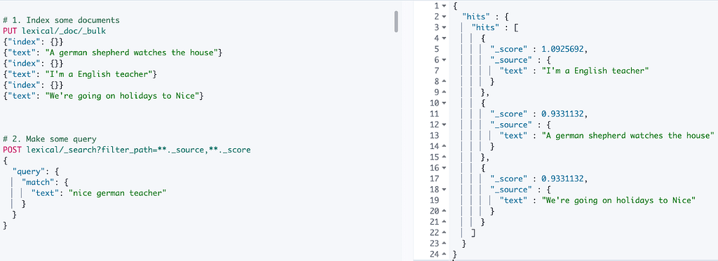
As we can see, the three documents to the top left are tokenized and analyzed. Then, the resulting terms are indexed in an inverted index, which simply maps the analyzed terms to the document IDs containing them. Note that all of the terms are only present once and none are shared by any document. Searching for “nice german teacher” will match all three documents with varying scores, even though none of them really catches the true meaning of the query.
As can be seen in Figure 2, below, it gets even trickier when dealing with polysemy or homographs, i.e., words that are spelled the same but have different meanings (right, palm, bat, mean, etc.) Let’s take the word “right” which can mean three different things, and see what happens.
Figure 2: Searching for homographs
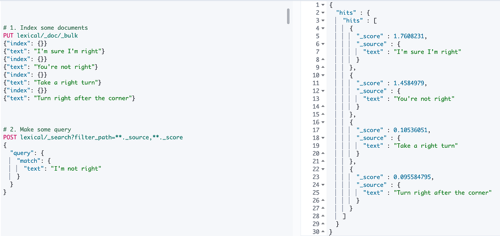
Searching for “I’m not right” returns a document that has the exact opposite meaning as the first returned result. If you search for the exact same terms but order them differently to produce a different meaning, e.g., “turn right” and “right turn,” it yields the exact same result (i.e., the third document “Take a right turn”). Granted, our queries are overly simplified and don’t make use of the more advanced queries such as phrase matching, but this helps illustrate that lexical search doesn’t understand the true meaning behind what’s indexed and what’s searched. If that’s not clear, don’t fret about it, we’ll revisit this example in the third article to see how vector search can help in this case.
To do some justice to lexical search, when you have control over how you index your structured data (think mappings, text analysis, ingest pipelines, etc.) and how you craft your queries (think cleverly crafted DSL queries, query term analysis, etc.), you can do wonders with lexical search engines, there’s no question about it! The track records of both OpenSearch and Elasticsearch regarding their lexical search capabilities are just amazing. What they’ve achieved and how much they have popularized and improved the field of lexical search over the past few years is truly remarkable.
However, when you are tasked to provide support for querying unstructured data (think images, videos, audios, raw text, etc.) to users who need to ask free-text questions, lexical search falls short. Moreover, sometimes the query is not even text, it could be an image, as we’ll see shortly. The main reason why lexical search is inadequate in such situations is that unstructured data can neither be indexed nor queried the same way as structured data. When dealing with unstructured data, semantics comes into play. What does semantics mean? Very simply, the meaning!
Let’s take the simple example of an image search engine (e.g., Google Image Search or Lens). You drag and drop an image, and the Google semantic search engine will find and return the most similar images to the one you queried. In Figure 3, below, we can see on the left side the picture of a German shepherd and to the right all the similar pictures that have been retrieved, with the first result being the same picture as the provided one (i.e., the most similar one).
Figure 3: Searching for a picture

Even if this sounds simple and logical for us humans, for computers it’s a whole different story. That’s what vector search enables and helps to achieve. The power unlocked by vector search is massive, as the world has recently witnessed. Let’s now lift the hood and discover what hides underneath.
Embedding vectors
As we’ve seen earlier, with lexical search engines, structured data such as text can easily be tokenized into terms that can be matched at search time, regardless of the true meaning of the terms. Unstructured data, however, can take different forms, such as big binary objects (images, videos, audios, etc.), and are not at all suited for the same tokenizing process. Moreover, the whole purpose of semantic search is to index data in such a way that it can be searched based on the meaning it represents. How do we achieve that? The answer lies in two words: Machine Learning! Or more precisely Deep Learning!
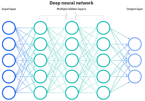
Deep Learning is a specific area of machine learning that relies on models based on artificial neural networks made of multiple layers of processing that can progressively extract the true meaning of the data. The way those neural network models work is heavily inspired by the human brain. Figure 4, below, shows what a neural network looks like, with its input and output layers as well as multiple hidden layers:
Figure 4: Neural network layers
The true feat of neural networks is that they are capable of turning a single piece of unstructured data into a sequence of floating point values, which are known as embedding vectors or simply embeddings. As human beings, we can pretty well understand what vectors are as long as we visualize them in a two or three-dimensional space. Each component of the vector represents a coordinate in a 2D x-y plane or a 3D x-y-z space.
However, the embedding vectors on which neural network models work can have several hundreds or even thousands of dimensions and simply represent a point in a multi-dimensional space. Each vector dimension represents a feature, or a characteristic, of the unstructured data. Let’s illustrate this with a deep learning model that turns images into embedding vectors of 2048 dimensions. That model would turn the German shepherd picture we used in Figure 3 into the embedding vector shown in the table below. Note that we only show the first and last three elements, but there would be 2,042 more columns/dimensions in the table.
embeddings |
Each column is a dimension of the model and represents a feature, or characteristic, that the underlying neural network seeks to modelize. Each input given to the model will be characterized depending on how similar that input is to each of the 2048 dimensions. Hence, the value of each element in the embedding vector denotes the similarity of that input to a specific dimension. In this example, we can see that the model detected a high similarity between dogs and German shepherds and also the presence of some blue sky.
In contrast to lexical search, where a term can either be matched or not, with vector search we can get a much better sense of how similar a piece of unstructured data is to each of the dimensions supported by the model. As such, embedding vectors serve as a fantastic semantic representation of unstructured data.
The secret sauce
Now that we know how unstructured data is sliced and diced by deep learning neural networks into embedding vectors that capture the similarity of the data along a high number of dimensions, we need to understand how the matching of those vectors works. It turns out that the answer is pretty simple. Embedding vectors that are close to one another represent semantically similar pieces of data. So, when we query a vector database, the search input (image, text, etc.) is first turned into an embedding vector using the same model that has been used for indexing all the unstructured data, and the ultimate goal is to find the nearest neighboring vectors to that query vector. Hence, all we need to do is figure out how to measure the “distance” or “similarity” between the query vector and all the existing vectors indexed in the database, that’s pretty much it.
Distance and similarity
Luckily for us, measuring the distance between two vectors is an easy problem to solve thanks to vector arithmetics. So, let’s look at the most popular distance and similarity functions that are supported by modern vector search databases, such as OpenSearch and Elasticsearch. Warning, math ahead!
L1 distance
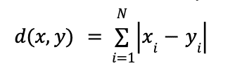
The L1 distance, also called the Manhattan distance, of two vectors x and y is measured by summing up the pairwise absolute difference of all their elements. Obviously, the smaller the distance d, the closer the two vectors are. The formula is pretty simple, as can be seen below:
Visually, the L1 distance can be illustrated as shown in Figure 4, below:
Figure 4: Visualizing the L1 distance between two vectors
Let’s take two vectors x and y, such as x = (1, 2) and y = (4, 3), then the L1 distance of both vectors would be | 1 – 4 | + | 2 – 3 | = 4.
L2 distance
The L2 distance, also called the Euclidean distance, of two vectors x and y is measured by first summing up the square of the pairwise difference of all their elements and then taking the square root of the result. It’s basically the shortest path between two points. Similarly to L1, the smaller the distance d, the closer the two vectors are:
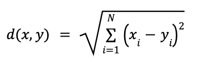
The L2 distance is shown in Figure 5 below:
Figure 5: Visualizing the L2 distance between two vectors
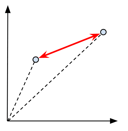
Let’s reuse the same two sample vectors x and y as we used for the L1 distance, and we can now compute the L2 distance as (1 – 4)2 + (2 – 3)2 = 10. Taking the square root of 10 would yield 3.16.
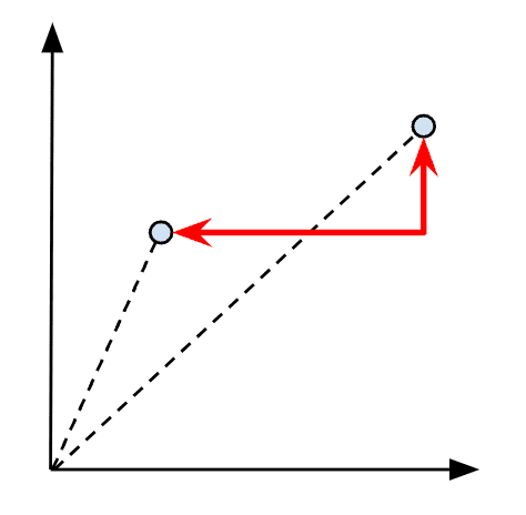
Linf distance
The Linf (for L infinity) distance, also called the Chebyshev or chessboard distance, of two vectors x and y is simply defined as the longest distance between any two of their elements or the longest distance measured along one of the axis/dimensions. The formula is very simple and shown below:
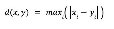
A representation of the Linf distance is shown in Figure 6 below:
Figure 6: Visualizing the Linf distance between two vectors
Again, taking the same two sample vectors x and y, we can compute the L infinity distance as max ( | 1 – 4 | , | 2 – 3 | ) = max (3, 1) = 3.
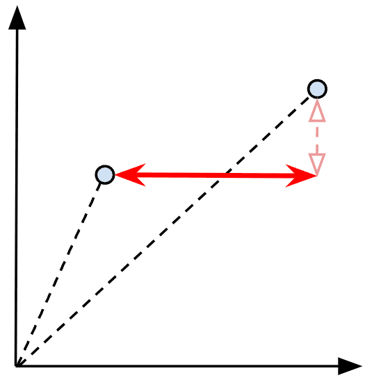
Cosine similarity
In contrast to L1, L2, and Linf, cosine similarity does not measure the distance between two vectors x and y, but rather their relative angle, i.e., whether they are both pointing in roughly the same direction. The higher the similarity s, the “closer” the two vectors are. The formula is again very simple and shown below:
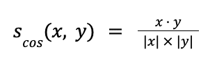
A way to represent the cosine similarity between two vectors is shown in Figure 7 below:
Figure 7: Visualizing the cosine similarity between two vectors
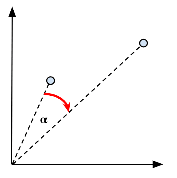
Furthermore, as cosine values are always in the [-1, 1] interval, -1 means opposite similarity (i.e., a 180° angle between both vectors), 0 means unrelated similarity (i.e., a 90° angle), and 1 means identical (i.e., a 0° angle), as shown in Figure 8 below:
Figure 8: The cosine similarity spectrum
Once again, let’s reuse the same sample vectors x and y and compute the cosine similarity using the above formula. First, we can compute the dot product of both vectors as (1・4) + (2 ・3) = 10. Then, we multiply the length (also called magnitude) of both vectors: (12 + 22)1/2 + (42 + 32)1/2 = 11.18034. Finally, we divide the dot product by the multiplied length 10 / 11.18034 = 0.894427 (i.e., a 26° angle), which is quite close to 1, so both vectors can be considered pretty similar.
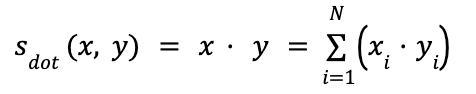
Dot product similarity
One drawback of cosine similarity is that it only takes into account the angle between two vectors but not their magnitude (i.e., length), which means that if two vectors point roughly in the same direction but one is much longer than the other, both will still be considered similar. Dot product similarity, also called scalar or inner product, improves that by taking into account both the angle and the magnitude of the vectors, which provides for a much more accurate similarity metric.
Two equivalent formulas are used to compute dot product similarity. The first is the same as we’ve seen in the numerator of cosine similarity earlier:
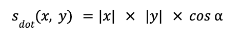
The second formula simply multiplies the length of both vectors by the cosine of the angle between them:
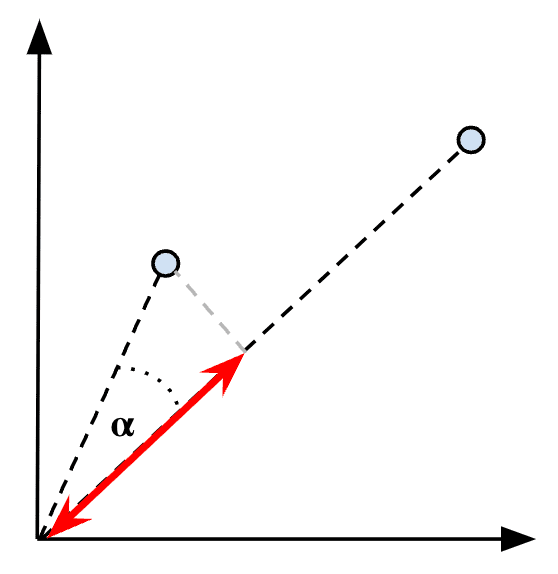
Dot product similarity is visualized in Figure 9, below:
Figure 9: Visualizing the dot product similarity between two vectors
One last time, we take the sample x and y vectors and compute their dot product similarity using the first formula, as we did for the cosine similarity earlier, as (1・4) + (2・3) = 10.
Using the second formula, we multiply the length of both vectors: (12 + 22)1/2 + (42 + 32)1/2 = 11.18034 and multiply that by the cosine of the 26° angle between both vectors, and we get 11.18034・cos(26°) = 10.
One thing worth noting is that if all the vectors are normalized first (i.e., their length is 1), then the dot product similarity becomes exactly the same as the cosine similarity (because |x| |y| = 1), i.e., the cosine of the angle between both vectors. As we’ll see later, normalizing vectors is a good practice to adopt in order to make the magnitude of the vector irrelevant so that the similarity simply focuses on the angle. It also speeds up the distance computation at indexing and query time, which can be a big issue when operating on billions of vectors.
Quick recap
Wow, we’ve been through a LOT of information so far, so let’s halt for a minute and make a quick recap of where we stand. We’ve learned that…
- …semantic search is based on deep learning neural network models that excel at transforming unstructured data into multi-dimensional embedding vectors.
- …each dimension of the model represents a feature or characteristic of the unstructured data.
- …an embedding vector is a sequence of similarity values (one for each dimension) that represent how similar to each dimension a given piece of unstructured data is.
- …the “closer” two vectors are (i.e., the nearest neighbors), the more they represent semantically similar concepts.
- …distance functions (L1, L2, Linf) allow us to measure how close two vectors are.
- …similarity functions (cosine and dot product) allow us to measure how much two vectors are heading in the same direction.
Now, the last remaining piece that we need to dive into is the vector search engine itself. When a query comes in, the query is first vectorized, and then the vector search engine finds the nearest neighboring vectors to that query vector. The brute-force approach of measuring the distance or similarity between the query vector and all vectors in the database can work for small data sets but quickly falls short as the number of vectors increases. Put differently, how can we index millions, billions, or even trillions of vectors and find the nearest neighbors of the query vector in a reasonable amount of time? That’s where we need to get smart and figure out optimal ways of indexing vectors so we can zero in on the nearest neighbors as fast as possible without degrading precision too much.
Vector search algorithms and techniques
Over the years, many different research teams have invested a lot of effort into developing very clever vector search algorithms. Here, we’re going to briefly introduce the main ones. Depending on the use case, some are better suited than others.
Linear search
We briefly touched upon linear search, or flat indexing, earlier when we mentioned the brute-force approach of comparing the query vector with all vectors present in the database. While it might work well on small datasets, performance decreases rapidly as the number of vectors and dimensions increase (O(n) complexity).
Luckily, there are more efficient approaches called approximate nearest neighbor (ANN) where the distances between embedding vectors are pre-computed and similar vectors are stored and organized in a way that keeps them close together, for instance using clusters, trees, hashes, or graphs. Such approaches are called “approximate” because they usually do not guarantee 100% accuracy. The ultimate goal is to either reduce the search scope as much and as quickly as possible in order to focus only on areas that are most likely to contain similar vectors or to reduce the vectors’ dimensionality.
K-Dimensional trees
A K-Dimensional tree, or KD tree, is a generalization of a binary search tree that stores points in a k-dimensional space and works by continuously bisecting the search space into smaller left and right trees where the vectors are indexed. At search time, the algorithm simply has to visit a few tree branches around the query vector (the red point in Figure 10) in order to find the nearest neighbor (the green point in Figure 10). If more than k neighbors are requested, then the yellow area is extended until the algorithm finds more neighbors.
Figure 10: KD tree algorithm
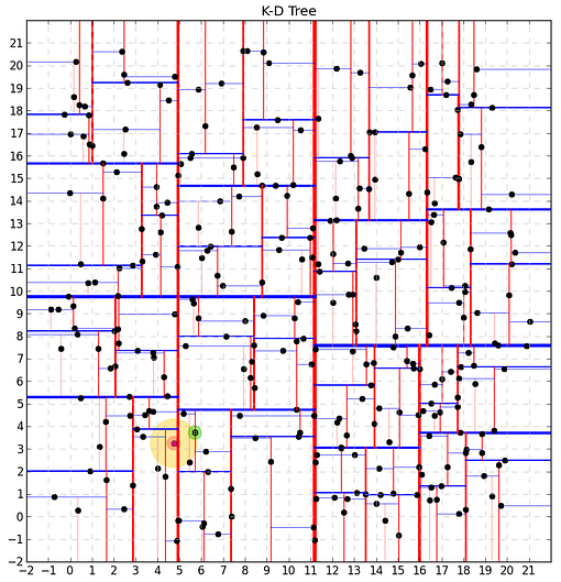
The biggest advantage of the KD tree algorithm is that it allows us to quickly focus only on some localized tree branches, thus eliminating most of the vectors from consideration. However, the efficiency of this algorithm decreases as the number of dimensions increases because many more branches need to be visited than in lower-dimensional spaces.
Inverted file index
The inverted file index (IVF) approach is also a space-partitioning algorithm that assigns vectors close to each other to their shared centroid. In the 2D space, this is best visualized with a Voronoi diagram as shown in Figure 11:
Figure 11: Voronoi representation of an inverted file index in the 2D space

We can see that the above 2D space is partitioned into 20 clusters, each having its centroid denoted as black dots. All embedding vectors in the space are assigned to the cluster whose centroid is closest to them. At search time, the algorithm first figures out the cluster to focus on by finding the centroid that is closest to the query vector, and then it can simply zero in on that area, and the surrounding ones as well if needed, in order to find the nearest neighbors.
This algorithm suffers from the same issue as KD trees when used in high-dimensional spaces. This is called the curse of dimensionality, and it occurs when the volume of the space increases so much that all the data seems sparse and the amount of data that would be required to get more accurate results grows exponentially. When the data is sparse, it becomes harder for these space-partitioning algorithms to organize the data into clusters. Luckily for us, there are other algorithms and techniques that alleviate this problem, as detailed below.
Quantization
Quantization is a compression-based approach that allows us to reduce the total size of the database by decreasing the precision of the embedding vectors. This can be achieved using scalar quantization (SQ) by converting the floating point vector values into integer values. This not only reduces the size of the database by a factor of 8 but also decreases memory consumption and speeds up the distance computation between vectors at search time.
Hierarchical Navigable Small Worlds (HNSW)
If it looks complex just by reading the name, don’t worry, it’s not really! In short, Hierarchical Navigable Small Worlds is a multi-layer graph-based algorithm that is very popular and efficient. It is used by many different vector databases, including Apache Lucene. A conceptual representation of HNSW can be seen in Figure 12, below.
Figure 12: Hierarchical Navigable Small Worlds
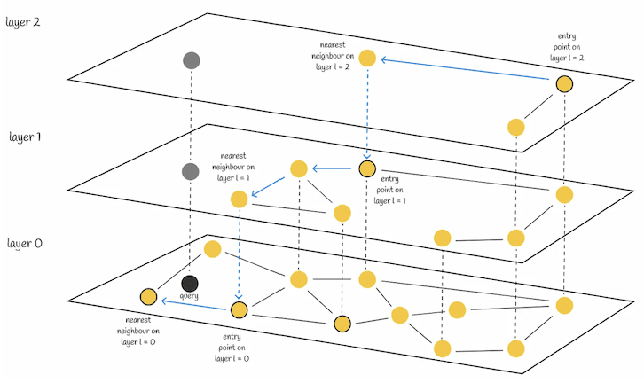
On the top layer, we can see a graph of very few vectors that have the longest links between them, i.e., a graph of connected vectors with the least similarity. The more we dive into lower layers, the more vectors we find and the denser the graph becomes, with more and more vectors closer to one another. At the lowest layer, we can find all the vectors, with the most similar ones being located closest to one another.
At search time, the algorithm starts from the top layer at an arbitrary entry point and finds the vector that is closest to the query vector (shown by the gray point). Then, it moves one layer below and repeats the same process, starting from the same vector that it left in the above layer, and so on, one layer after another, until it reaches the lowest layer and finds the nearest neighbor to the query vector.
Locality-sensitive hashing (LSH)
In the same vein as all the other approaches presented so far, locality-sensitive hashing seeks to drastically reduce the search space in order to increase the retrieval speed. With this technique, embedding vectors are transformed into hash values, all by preserving the similarity information, so that the search space ultimately becomes a simple hash table that can be looked up instead of a graph or tree that needs to be traversed. The main advantage of hash-based methods is that vectors containing an arbitrary (big) number of dimensions can be mapped to fixed-size hashes, which enormously speeds up retrieval time without sacrificing too much precision.
There are many different ways of hashing data in general, and embedding vectors in particular, but this article will not dive into the details of each of them. Conventional hashing methods usually produce very different hashes for data that seem very similar. Since embedding vectors are composed of float values, let’s take two sample float values that are considered to be very close to one another in vector arithmetic (e.g., 0.73 and 0.74) and run them through a few common hashing functions. Looking at the results below, it’s pretty obvious that common hashing functions do not retain the similarity between the inputs.
0.73 | ||
|---|---|---|
Let’s conclude
In order to introduce vector search, we had to cover quite some ground in this article. After comparing the differences between lexical search and vector search, we’ve learned how deep learning neural network models manage to capture the semantics of unstructured data and transcode their meaning into high-dimensional embedding vectors, a sequence of floating point numbers representing the similarity of the data along each of the dimensions of the model. It is also worth noting that vector search and lexical search are not competing but complementary information retrieval techniques (as we’ll see in the third and fifth parts of this series when we’ll dive into hybrid search).
After that, we introduced a fundamental building block of vector search, namely the distance (and similarity) functions that allow us to measure the proximity of two vectors and assess the similarity of the concepts they represent.
Finally, we’ve reviewed different flavors of the most popular vector search algorithms and techniques, which can be based on trees, graphs, clusters, or hashes, whose goal is to quickly narrow in on a specific area of the multi-dimensional space in order to find the nearest neighbors without having to visit the entire space like a linear brute-force search would do.
If you like what you’re reading, make sure to check out the other parts of this series:
- Part 2: How to Set Up Vector Search in OpenSearch
- Part 3: Hybrid Search Using OpenSearch
- Part 4: How to Set Up Vector Search in Elasticsearch
- Part 5: Hybrid Search Using Elasticsearch