
Quick Links
- Introduction
- How do you like your vectors?
- How to set up the k-NN plugin
- How to set up the Neural Search plugin
- Pros and cons of each approach
- Let’s conclude
Introduction
This article is the second in a series of five that dives into the intricacies of vector search (aka semantic search) and how it is implemented in OpenSearch and Elasticsearch.
The first part: A Quick Introduction to Vector Search, was focused on providing a general introduction to the basics of embeddings (aka vectors) and how vector search works under the hood. The content of that article was more theoretical and not oriented specifically on OpenSearch, which means that it was also valid for Elasticsearch as they are both based on the same underlying vector search engine: Apache Lucene.
Armed with all the vector search knowledge learned in the first article, this second article will guide you through the meanders of how to set up vector search in OpenSearch using either the k-NN plugin or the new Neural Search plugin that was recently made generally available in 2.9.
In the third part: OpenSearch Hybrid Search, we’ll leverage what we’ve learned in the first two parts and build upon that knowledge by delving into how to craft powerful hybrid search queries in OpenSearch.
The fourth part: How to Set Up Vector Search in Elasticsearch and the fifth part: Elasticsearch Hybrid Search, will be similar to the second and third ones but focused on Elasticsearch.
How do you like your vectors?
Before getting too technical, we need to introduce the two flavors of semantic search supported by OpenSearch.
The first option is to leverage the k-NN plugin (k-nearest neighbors) which has been available since version 1.0. k-NN enables searching for the k-nearest neighbors to a query vector across an index of vectors. Neighbors are determined by measuring the distance or similarity between two points in a given multi-dimensional vector space. The shorter the distance between two points, the closer the semantic meaning of the two related vectors.
The second option is to use the new Neural Search plugin which has been in preview since version 2.5 and was recently made generally available in version 2.9. As we’ll see later in this article, the Neural Search plugin is just a wrapper around the k-NN plugin. Its main advantage is that it works on pre-trained Machine Learning models that can generate text embeddings on the fly, both at ingestion and search time, which is not the case for the k-NN plugin which requires you to create the embeddings using an ad-hoc client library.
Both of these plugins work on the exact same data type called `knn_vector` which we’re going to explain how to set up next.
How to set up the k-NN plugin
In order for k-NN search to work, we must first create an index that defines at least one field of type `knn_vector` which is where your vector data will be stored. There are two ways of defining `knn_vector` fields, either by using a model or with a method definition, and the method we select basically determines and configures the approximate k-NN algorithm we will use. We’re going to handle the latter first because the former relies on it too.
Using a method definition
The mapping below shows a `knn_vector` field called `my_vector` of dimension 4. The field will use the `nmslib` engine with the `hnsw` method.
"my_vector": {
  "type": "knn_vector",
  "dimension": 4,
  "method": {
    "engine": "nmslib",
    "name": "hnsw",
    "space_type": "l2",
    "parameters": {
      "ef_construction": 128,
      "m": 24
    }
  }
}
It might look ungraspable at this point, but don’t worry as we’re going to dive into the details shortly. We just need to explain some terminology first. The `method.engine` setting relates to the k-NN library that we want to use for indexing and search. There are currently three available libraries: `nmslib`, `faiss`, and `Lucene`.
Each of those libraries supports different methods (i.e., the `method.name` setting), which represent different algorithms for creating and indexing the vector data, and each of those methods has its own set of supported spaces (i.e., the `method.space_type` setting) and configuration parameters (i.e., the `method.parameters` setting). The table below summarizes all available engines and their supported method definitions and spaces as well as their related configuration parameters:
Table 1: The different method definitions and their configuration parameters
| Engi-nes | Meth-ods | Train-ing | Spaces | Method params | Enco-ders | Encoder training | Encoder params |
| nmslib | hnsw | No | l1 l2 linf innerproduct cosinesimil | ef_constructionm | |||
| faiss | hnsw | No | l2 innerproduct | ef_construction ef_search | |||
| encoder | flat | No | |||||
| pq | Yes | m code_size | |||||
| ivf | Yes | l2 innerproduct | nlist nprobes | ||||
| encoder | flat | No | |||||
| pq | Yes | m code_size | |||||
| Lucene | hnsw | No | l2 cosinesimil | ef_constructionm |
As can be seen in Table 1, the `hnsw` method has been implemented by all engines. `hnsw` stands for Hierarchical Navigable Small Worlds and is a very popular, robust, and fast algorithm for approximate nearest neighbors search as we’ve seen in the preceding article of this series. `ivf`, which stands for Inverted File System, is another algorithm supported by the `faiss` engine. It’s beyond the scope of this article to delve into the details of these two algorithms, but there are interesting resources out there that deal with these topics, such as this one from AWS.
Another important topic to touch upon is spaces. A space basically corresponds to the function we use to measure the distance between two points in order to determine the k-nearest neighbors. You can refer to our first article where we spent quite some time describing all the distance functions available for approximate k-NN search. Also, you can find some additional information regarding distance functions in the official OpenSearch documentation.
We’ll also not dive into the details of each of the method parameters here (`ef_construction`, `m`, etc.), we simply invite you to check out the official OpenSearch documentation which describes them very well.
To wrap up, Table 2 below summarizes all the mapping parameters that can be specified when defining a `knn_vector` field using a method definition.
Table 2: The mapping definition of `knn_vector` fields using a method definition
| Setting name | Required | Default | Description |
|---|---|---|---|
| dimension | Yes | - | The number of dimensions of the vector data |
| method.engine | No | nmslib | The k-NN library to use for indexing and search |
| method.name | Yes | - | The algorithm to use to create the vector index |
| method.space_type | No | l2 | The distance function to measure the proximity of two points in the vector space |
| method.parameters | No | - | The parameters of the used method |
At this point, all the potential combinations might feel overwhelming, and it can be hard to know which engine, method, space, and parameters to pick to define your vector field mapping. Fear not, we’ll dive into this right after the next section, where we introduce the second way of defining `knn_vector` fields using models.
Using a model
As just mentioned, we’ll provide a few directions on how to pick the best engine and method for your use case in a bit, but for now, let’s just assume that we’ve picked a method definition that requires some training first. According to Table 1, that would mean the `faiss` engine either with 1) the `ivf` method definition or 2) any method that uses a `pq` encoder (short for “product quantization,” which we briefly touched upon in the first article).
When defining a `knn_vector` field using a model, the mapping definition becomes very straightforward and simply contains the ID of the trained model, as shown in the code below:
"my_vector": {
  "type": "knn_vector",
  "model_id": "my-trained-model"
}
Now, what do we need to do before we can create an index using this method? You guessed it! We need to create a model and train it in order to be able to reference it in the field mapping. This trained model will then be used to initialize the native library index (i.e., `faiss`) during each segment creation of the index.
In order to create such a model, we can use the OpenSearch Train API by specifying an index containing the training data as well as the method definition to use. Let’s proceed step-by-step; we need to:
- Create an index to hold the training data and load it
- Source that index to train the model as specified by a given method definition (e.g., `faiss` + `ivf`)
- Create the main index with the `knn_vector` field that references the created model ID.
1. Create the index to hold training data and load it
In order to create the index to store the training data, we just have to define a `knn_vector` field with a specific dimension, which will become the dimension of the model that will be created:
# 1. Create a simple index with a knn_vector field of dimension 3
PUT /my-training-index
{
  "settings": {
    "number_of_shards": 1,
    "number_of_replicas": 0
  },
  "mappings": {
    "properties": {
      "my_training_field": {
        "type": "knn_vector",
        "dimension": 3
      }
    }
  }
}

# 2. Load that index with training data
POST my-training-index/_doc/_bulk
{ "index": { "_id": "1" } }
{ "my_training_field": [2.2, 4.3, 1.8]}
{ "index": { "_id": "2" } }
{ "my_training_field": [3.1, 0.7, 8.2]}
{ "index": { "_id": "3" } }
{ "my_training_field": [1.4, 5.6, 3.9]}
{ "index": { "_id": "4" } }
{ "my_training_field": [1.1, 4.4, 2.9]}
2. Train the model
After the training index has been created and loaded with data, we can call the Train API in order to create the model that we call `my-trained-model`. In the `_train` call, we specify the following parameters:
- `training_index`: the name of the training index we’ve just created
- `training_field`: the name of the field in the training index that contains the vector data to use for the training
- `dimension`: the dimension of the model to create, which must be the same as the vector dimension in the training index
- `method`: the method definition (i.e., `faiss` engine + `ivf` algorithm) that must be used to build the model as previously described in Table 1.
POST /_plugins/_knn/models/my-trained-model/_train
{
  "training_index": "my-training-index",
  "training_field": "my_training_field",
  "dimension": 3,
  "description": "My model description",
  "method": {
    "engine": "faiss",
    "name": "ivf",
    "space_type": "l2",
    "parameters": {
      "nlist": 4,
      "nprobes": 2
    }
  }
}
When the `_train` call returns, the model starts to build. You can retrieve the details about the model being created using the following command:
GET /_plugins/_knn/models/my-trained-model

=> Returns
{
  "model_id": "my-trained-model",
  "model_blob": "SXdGbA…AAAAAA=",
  "state": "created",
  "timestamp": "2023-08-18T09:21:37.180220737Z",
  "description": "My model description",
  "error": "",
  "space_type": "l2",
  "dimension": 4,
  "engine": "faiss"
}
Once the `state` is `created`, your model is ready to use and we can proceed to the last step, i.e., creating the main index where the `knn_vector` field can be defined using the trained model.
3. Create the main index
Now, we can finally create our main index with a `knn_vector` field called `vector-field` defined by the model `my-trained-model` that we’ve just created. Also note that this index must have `index.knn: true` specified in the index settings to indicate that the index should build native library indexes so that vector fields can be searched.
Note: We didn’t specify this setting when creating the training index because we only wanted to store vector data for training purposes, not for search.
PUT /main-index
{
  "settings": {
    "number_of_shards": 3,
    "number_of_replicas": 1,
    "index.knn": true
  },
  "mappings": {
    "properties": {
      "vector-field": {
        "type": "knn_vector",
        "model_id": "my-trained-model"
      }
    }
  }
}
Voilà! Once `main-index` is loaded with our data, it will be ready to support k-NN search queries, but that is the subject of another article that you can check out.
Before switching to the Neural Search plugin, we promised to give some directions regarding how to go about picking the right engine, method, space, and parameters when defining your vector fields.
Picking the right method
There are many possible combinations to choose from when defining your vector fields. However, there are a few directions that we can provide depending on how you intend to use your vector data. You need to thoroughly understand your requirements but also be ready to make some trade-offs. The four main factors you need to consider are the following:
- Query latency
- Query quality
- Memory limits (here are some instructions for estimating your memory usage)
- Indexing latency.
First, if you’re not too concerned about memory usage, `hnsw` offers a very strong trade-off between query latency and query quality. In other words, fast search speeds and fantastic recall. Indexing latency, however, is not the fastest.
If you don’t want to use too much memory but index faster than `hnsw`, with similar query quality, you should evaluate `ivf`. Remember, however, that this will require you to go through a training step to build a model.
If you’re really concerned about memory usage, consider using the `faiss` engine with either the `hnsw` or `ivf` algorithm but configured with a `pq` encoder. Because `pq` is a lossy encoding, the query quality will drop.
If you care about reducing both your memory and storage footprint in exchange for a minimal loss of recall, you can opt for the `lucene` engine and replace `float` vectors with `byte` vectors. As a float takes up four times as many bits as a byte, you can drastically reduce the storage needed to store your vector data. This possibility has been available since version 2.9 and can be configured by adding the `data_type` parameter (`byte` or `float`) in the field mapping definition.
If your vectors are already normalized (i.e., their length is 1), you should prefer using the `innerproduct` space type (i.e., similarity function) as the computation will be carried out much faster than with `cosinesimil`. Note, however, that `innerproduct` is not available for the `lucene` engine.
Even though the directions above give a pretty good idea of what to pick, nothing beats testing! Make sure to identify a few potential methods that could work for your use case and then test, test, test on your own data set.
How to set up the Neural Search plugin
The Neural Search plugin also leverages the `knn_vector` data type together with pre-trained text-embedding Machine Learning (ML) models that can generate embeddings on the fly. Hence, prior to creating our index, we first need to load such a text-embedding model. We have a few options:
- Use a pre-trained model available natively in OpenSearch
- Use any model available online, such as on the popular Huggingface repository
- Use a custom model.
In this article, we’ll only handle the first option to give a general idea of how this works. The other two options might be the subject of a future article.
Use a pre-trained model
As of version 2.9, there are nine available pre-trained models provided natively by OpenSearch. Each of them has its own specificities (dimensions, training content, data size, etc.), and it might be worth checking them out to decide which one best suits your needs.
For the purpose of this article, we’ve chosen the `all-MiniLM-L6-v2` model available on Huggingface. The steps required to use it are as follows:
- Upload the ML model into your cluster
- Deploy the ML model
- Define an ingest pipeline to create embeddings on the fly
- Create an index to store your vector data.
1. Upload the model
Uploading the model is very simple and requires a simple call to the Upload Model API:
POST /_plugins/_ml/models/_upload
{
  "name": "huggingface/sentence-transformers/all-MiniLM-L6-v2",
  "version": "1.0.1",
  "model_format": "TORCH_SCRIPT"
}

Returns =>
{
  "task_id": "nPQV2YkB8n-uOBQ59r9s",
  "status": "CREATED"
}
The response is returned immediately and contains a task ID that can be used to monitor the progress of the model uploading process that is running in the background:
GET _plugins/_ml/tasks/nPQV2YkB8n-uOBQ59r9s

Returns =>
{
  "model_id": "O7IV2YkBFKz6Xoem-EFU",
  "task_type": "REGISTER_MODEL",
  "function_name": "TEXT_EMBEDDING",
  "state": "COMPLETED",
  "worker_node": [
    "SONz3jdOT4K1RPmsXfTkHw"
  ],
  "create_time": 1691564242539,
  "last_update_time": 1691564269003,
  "is_async": true
}
2. Deploy the model
Once the task state is `COMPLETED`, the response will contain a `model_id` that can be used to load and deploy the model. By hitting the Load Model API, we can load and deploy the model into memory:
POST /_plugins/_ml/models/O7IV2YkBFKz6Xoem-EFU/_load

Returns =>
{
  "task_id": "uPQZ2YkB8n-uOBQ5hb_D",
  "status": "CREATED"
}
Again, the response contains a task ID that can be used to monitor the progress of the model loading that is running in the background. When the state turns to `RUNNING`, the model has been deployed and is ready to be used:
GET _plugins/_ml/tasks/uPQZ2YkB8n-uOBQ5hb_D

Returns =>
{
  "model_id": "O7IV2YkBFKz6Xoem-EFU",
  "task_type": "DEPLOY_MODEL",
  "function_name": "TEXT_EMBEDDING",
  "state": "RUNNING",
  "worker_node": [
    "D_I8VQ6DSRyNep-iXLfHPg",
    "b-KkZEbbRkSgUVYp6-wNZw",
    "zjoBBDXHTS-y0z8VqolTmw",
    "SONz3jdOT4K1RPmsXfTkHw",
    "jVx-_UgsTr--XdSB05vyoQ",
    "dhu-d03oQpqBTgYIlAp3mg"
  ],
  "create_time": 1691564475841,
  "last_update_time": 1691564476005,
  "is_async": true
}
3. Define an ingest pipeline
Now that the pre-trained model has been uploaded and deployed, we can use it in an ingest pipeline to generate embeddings on the fly. The ingest pipeline called `embeddings-pipeline` contains a single `text_embedding` processor that uses the model we’ve just uploaded and deployed in order to generate embeddings for the content found in `text-field` and store it in `vector-field`:
PUT _ingest/pipeline/embeddings-pipeline
{
  "description": "Provides support for generating embeddings",
  "processors" : [
    {
      "text_embedding": {
        "model_id": "O7IV2YkBFKz6Xoem-EFU",
        "field_map": {
           "text-field": "vector-field"
        }
      }
    }
  ]
}
Quick note: The `text_embedding` processor is similar to and does the same job as the `inference` processor provided by Elasticsearch.
4. Create the main index
Now that our ingest pipeline has been created, we can finally create the index to store the vector data we want to be able to search. Again, we enable the `index.knn` setting but also specify the `index.default_pipeline` setting to make sure that all documents that we are going to index will go through the ingest pipeline to have their embeddings generated automatically.
On the mapping side, we have one field called `text-field` of type `text` which will contain the main text content, and `vector-field` of type `knn_vector`. We define the vector field with 384 dimensions, i.e., the same number of dimensions as the `all-MiniLM-L6-v2` model. Regarding the method definition, we’ve used the `lucene` engine with the `hnsw` algorithm.
Also, it is worth noting that even though the vectors generated by the model are normalized (i.e., of length 1), we cannot use the `innerproduct` space type as it is not supported by the `lucene` engine, so we simply use the `cosinesimil` one, which will do the job:
PUT /main-index
{
  "settings": {
    "index.knn": true,
    "index.default_pipeline": "embeddings-pipeline"
  },
  "mappings": {
    "properties": {
      "text-field": {
        "type": "text"
      },
      "vector-field": {
        "type": "knn_vector",
        "dimension": 384,
        "method": {
          "name": "hnsw",
          "space_type": "cosinesimil",
          "engine": "lucene"
        }
      }
    }
  }
}
Loading the index is pretty simple because we only need to provide the text content and the embeddings will be generated on the fly at ingest time and indexed into the internal `hnsw` index managed by the `lucene` engine:
POST main-index/_doc/_bulk
{ "index": { "_id": "1" } }
{ "text-field": "The big brown fox jumps over the lazy dog"}
{ "index": { "_id": "2" } }
{ "text-field": "Lorem ipsum dolor"}
Voilà again! Our index can now serve semantic search queries based on vector data. Even though that is the subject of the next article of this series, we would like to quickly show you what such a query would look like. Because, thanks to the model, there is no need to provide the text embeddings of the searched content, the query is also generated on the fly by the model at search time.
5. Query the index
In the query below, we can see that we make use of the `neural` search query to search the `vector-field` using the ML model that we loaded earlier. The text embedding for the question “Who jumps over a dog?” is generated on the fly at search time, which makes the query payload much smaller depending on how many dimensions your vectors have. Of course, since the embeddings are now generated on the fly at search time, that will increase the search latency of the query a little bit, though that increase should be negligible.
POST main-index/_search
{
  "size": 3,
  "_source": [
    "text-field"
  ],
  "query": {
    "bool": {
      "must": [
        {
          "neural": {
            "vector-field": {
              "query_text": "Who jumps over a dog?",
              "model_id": "O7IV2YkBFKz6Xoem-EFU",
              "k": 3
            }
          }
        }
      ]
    }
  }
}
As mentioned earlier in this article, under the hood, the `neural` search query is just a wrapper around a `knn` query. The specified ML model is used instead of an ad hoc embeddings generator (e.g., OpenAI, Cohere, etc.) in order to create the embeddings vector corresponding to the provided query text. As such, the above `neural` query is equivalent to the following `knn` query where the query `vector` parameter contains the embeddings vector representing the query text “Who jumps over a dog?” as generated by the model `O7IV2YkBFKz6Xoem-EFU`:
POST main-index/_search
{
"size": 3,
"_source": [
"text-field"
],
"query": {
"bool": {
"must": [
{
"knn": {
"vector-field": {
"vector": [0.23, 0.17, ..., 0.89, 0.91],
"k": 3
}
}
}
]
}
}
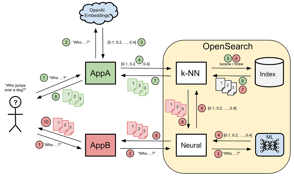
}Figure 1, below, illustrates how both plugins work and how the Neural Search plugin leverages the local ML model and the k-NN plugin in order to do its job. We can see two applications: A (green path) uses the k-NN plugin and B (red path) utilizes the new Neural Search plugin. The main difference is that application A needs to resort to an ad hoc embeddings generator (OpenAI, Cohere, etc.), while application B does the same job using an internal ML model. Ultimately, the k-NN plugin ends up receiving the embeddings query vector and finding the nearest neighbors.
Figure 1: Interactions between two applications using the k-NN and Neural Search plugins
A more concrete example
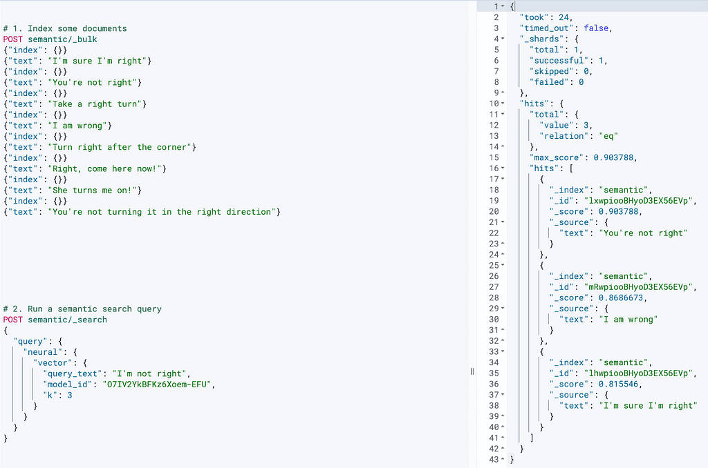
Remember the “I’m not right” example from the first article? Let’s see how the `neural` search query can help us retrieve more accurate results. We’ve added some more documents, one of which is “I am wrong.”
Figure 2, below, shows that searching for “I’m not right” using the `neural` semantic search query instead of a normal lexical `match` query now returns a much more accurate result, namely “You’re not right” and “I am wrong,” which is exactly what we were expecting. It is also worth noting that “I am wrong” is not even returned by a normal lexical search since there are no matching tokens.
Figure 2: Neural search query returning more accurate results
In the third article, we’ll revisit this example and see how the new `hybrid` search query can help return even more accurate results.
Pros and cons of each approach
Both approaches to semantic search described in this article have pros and cons. Depending on your precise use case and constraints, you might decide to pick one or the other. If you pick Neural Search, you might have to first find the right NLP model to support your needs, which might not be trivial. The table below lists the main pros and cons of each approach:
| k-NN plugin | Neural Search plugin | |
|---|---|---|
| Pros | - Available natively in OpenSearch since OS 1.0 - Very simple to set up - Very simple to use and supports approximate k-NN, exact (aka brute force) k-NN, and Painless extensions. | - Available natively in OpenSearch since OS 2.5 (GA in 2.9) - The queries accept free-text user input, which also makes them much smaller - The embeddings are generated internally by the pre-trained model - No additional cost for generating embeddings - Depending on the chosen pre-trained model, the number of dimensions is lower than 1024, which allows the use of the Lucene vector engine |
| Cons | - The knn query doesn’t yet support pre-filtering, script_score does though - An additional step is required to generate the embeddings on the client side (both at indexing and search time) - An additional cost can be incurred for generating the embeddings (e.g., from the OpenAI Embeddings API) - The number of dimensions is dictated by the embeddings API or generator being used (e.g., 1536 for OpenAI which can be considered high) - Bigger query payload due to the fact that a vector of 1536 float values needs to be passed every time. | - The neural search query doesn’t yet support pre-filtering - The required setup of an arbitrary ML model taken anywhere online is a bit more involved than for a pre-trained one - Finding the right model (and potentially training it) can be a non-trivial task. |
Let’s conclude
In this article, we’ve introduced the two vector search plugins supported by OpenSearch, namely the k-NN and Neural Search plugins.
We delved into the former and explained how to set it up using either a model or a method definition. For each method, we went over the different supported engines and the algorithms they implement as well as the configuration parameters that are expected. In case you pick a method that requires pre-training, we’ve explained how to load data into a temporary index and how to train a model so that you can then load your main index with vector data. More importantly, we also quickly reviewed some guidelines on how to pick the best method depending on your use case and constraints.
Regarding the Neural Search plugin, which mainly works in concert with ML models, we’ve demonstrated how to upload and deploy a pre-trained model, how to create an ingest pipeline that leverages this model, and how to load your index using this ingest pipeline. Finally, we showed a simple use case with the `neural` search query.
We concluded by listing the most important pros and cons of each approach. We hope that this article was insightful and that you had a pleasant experience going through it and testing it out on your OpenSearch cluster.
If you like what you’re reading, make sure to check out the other parts of this series:
- Part 1: A Quick Introduction to Vector Search
- Part 3: Hybrid Search using OpenSearch
- Part 4: How to Set Up Vector Search in Elasticsearch
- Part 5: Hybrid Search Using Elasticsearch